Introduction to Naïve Bayes in Cybersecurity

Introduction to Naïve Bayes in Cybersecurity
With the increasing threat of cybersecurity attacks, we are seeing the rise of security analytics, and where systems such as Splunk, QRadar and HPE Arcsight are used to collect, analyse and detect threats. Normally human analysts are used to make sense of the alerts created, but they are often increasingly overloaded by the number of alerts and possible threats. Thus machine learning can be used to make sense of the alerts and correlate these together, and then pass the results onto human analysts.
Machine Learning
For Machine Learning (ML) there are typically two main phases: training and testing, with a common set of steps of defining the features and classes within the training data set. Next a subset of attributes is located for classification, and a learning model applied on the training data. With the learning model, the rest of the data is then fitted back, and the success rate determined. The basic process that we have in applying machine learning to cyber security is:
- Information sources. This involves defining the sources of information that would be required to capture the right information.
- Data capturing tools. This involves creating the software agents required to the required data.
- Data pre-processing. This involves processing the data into a format which is ready for the analysis part.
- Feature extraction. This involves defines the key features that would be required to the analysis engine.
- Analysis engine. This involves the creation of an analysis engine which takes the features and creates scoring to evaluate risks.
- Decision engine. This takes the scoring systems from the analysis stage and makes a reasoned decision on the level of risk involved.
Success criteria
The two main approaches used within the detection of threats is within signature detection, where we match against well-known patterns of malicious behaviour, or use anomaly detection, where we define a normal behavior pattern, and then detect deviations away from this. For machine-focused threats, such as for viruses and worms, the signature methods are best, but for the detection of human focused zero-day threats and for, such as for fraud and data theft, the anomaly detection methods normally work best.
Within machine learning there are often two main phases: training and testing. This involves defines the class attributes (features) and classes from training data, and then to reduce these to a subnet which can be used within the classification process. A model is then created with the training set, and where the model is then used on the complete data set in order to understand the success rate. This output may be in the form of a metric or a decision. When it is a decision we typically define a confusion matrix approach where we measure the predicted values against the actual values. For example we may have a detection system which monitors and classifies user logins, and we can draw a confusion matrix to show the success rates:

Within a decision engine, we often use the concept of correct guesses (true) and incorrect ones (false). So, a true positive is where we determine that an event was correctly detected, while a false positive is where a true event was not detect (and thus missed by the system). Within IDS (Intrusion Detection Systems) there is often a balance to be struck when tuning the systems so that users do not get swamped by too many false alerts (false positives), or from too many fake alerts.
Elements of a machine learning package
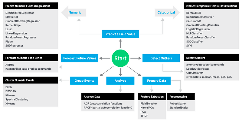
Splunk is one of the most successful packages for Cybersecurity analytics, and defines seven main elements for machine learning (Figure 1):
- Preprocessing: This defines how the data is scaled to produce the correct range (such as for numerical values to be scaled to a given range). A typical method is StandardScalar.
- Feature Extraction: This defines a method to extract key features that are required for the machine to learn on. Typical methods are PCA (Principle Component Analysis) and TFIDF.
- Analysing data: This involves analysing the correlations between data. Typical methods include ACF (autocorrelation factors) and PACF (partial autocorrelation factors).
- Classification: This involves classifying data into groups. Typical methods include: SVM and RandomForestClassifier.
- Group events: This normally involves clustering. Kmeans and BIRCH are typical methods.
- Detection of outliers: This defines anomalies within the data sets, and be used in anomaly detection. A typical method is OneClassSVM.
- Prediction: This makes predictions on the data given a set of known inputs, and can either be numerical predictions (such as using linear regression, random forest regression, lasso, and decision tree regression) or categorical (such as with logistic regression).
- Forecasting: This defines a method to predict future data values from the history of the data. Typical methods are ARIMA (Autoregressive integrated moving average) and KalmanFilter.
Naïve Bayes
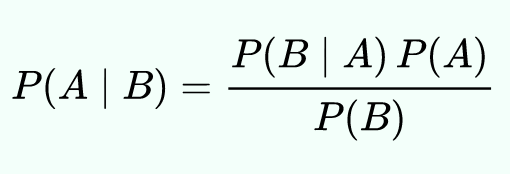
The Naïve Bayes classification method is based on Bayes’ theorem, and relates to the independent nature of predictors (non-related features). For this we have P(A | B), and which is the probability of an Event A given B; P(B | A), which probability of Event B given A; P(A) the likelihood of Event A; and P(B) the likelihood of Event B. The theorem then defines:
For example, if we monitor our systems (A), and detect the following hacks (B):

We can see that we have 15 attacks recorded. First, we can produce a frequency table for the attacks against our systems:

We can now see that P(Sales)=0.467 (7/15), P(Production)=0.267 (4/15) and P(R&D)=0.333 (5/15), and that P(Phishing)=0.64, P(Crypto crack)=0.18 and P(Network attack)=0.45. And, so we have a probability that our Sales server will be hacked for 46.7% of the time, and the probability that it is a network attack is 33.3% of the time. Next, we can define the probability of A (System) occurring given B (Attack Type), and which is P(A|B). For this we simply take each attack, and then divide by the total number of these attacks:

In this case we see:

Thus the probability that it is the Sales server that has been hit if we know we have a phishing attack is 0.429. If we know that it is a crypto attack, there is a 50/50 chance between the Sales server and the R&D server. The sum of our probabilities of knowing B (the attack) to determine P(A|B) should equal unity.
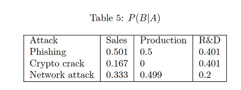
Now we will use Bayes logic to determine P(B | A), and where we can determine the probability of the attack type (A) given the server (B). Thus for:

We can then determine the following:
In Bayes, we need strong independence between events A and B.
Within the scikit-learn we can use three naive Bayes probabilistic distributions:
- Bernoulli. This defines a basic binary classification as to whether a feature is present or not.
- Multinomial. This defines a discrete measure of the strength of a feature.
- Gaussian. This defines both a mean and variance of the strength of a feature.
So let’s say that we have a phishing email detector, and we take samples and determine the number of characters in the subject field, and the number of words in the email. Let say that the samples for true phishing are (subject_field_characters=34,words=100), (80,230), and (70,400), and the samples for not phishing are (55,20), (38,30), (20,25) and (18,40). In case the first variable is the number of characters in the subject field, and the second one is the number of words in the email. We can now go ahead and define these, and use a GaussianNB() classifier, and then fit:
Next we can score the success of the model, and try out some sample values:
print binary_class.score(X, Y)
data = np.array([[28, 30], [40, 100], [4, 500], [10, 10]])
print binary_class.predict(data)
In this case we get:
Samples
[[ 34 100]
 [ 80 230]
 [ 70 400]
 [ 55 20]
 [ 28 30]
 [ 20 25]
 [ 18 40]]
[1 1 1 0 0 0 0]
Score = 1.0
Classification = [0 1 1 0]
And where the classifier has identified that (28, 30) and (10, 10) are not phishing emails, and (40, 100), (4, 500) are.
Conclusions
Bayes methods are useful when there are independent variables, and where these can be used to benchmark probabilities. These can then be used to detect anomalies on the system.