If You’re Into Cybersecurity, Get Into Splunk and Machine Learning

If You’re Into Cybersecurity, Get Into Splunk and Machine Learning

The future will see the rise of the cybersecurity specialist who uses data science and machine learning in the way that we have used speadsheets in the past. These specialists will be able to take data sets from logs on systems and from open source data sets, and then make predictions on the data. They will find the correlations and build new threat models. The rise of Splunk, too, seems almost endless, especially as it provides a great interface to machine learning models.

So let’s take an example for malware infection [download dataset]:

The data set we have contains 98,944 records, which is rather a lot, so we will just analyse the first 50,000. Overall the fields used are: receive_time, serial_number, session_id, src_ip, dst_ip, bytes_sent, bytes_received, packets_sent, packets_received, dest_port, src_port, used_by_malware, and has_known_vulnerability. First we will use the logistic regression learning method in order to train on “used_by_malware”) and against all the other fields:

In machine learning, we normally do a 70/30% split and where we train on 70% of the data, and then test against the remaining 30%. In this case we will use a simple logicistic regression model with a 70/30 split:

Next, in Splunk, we select the Train Model button, and wait for a minute or so. Our results are then:

This creates a model defined by “example_malware”. Next we can simply view the confusion matrix with (or click on the Classification Results link):

| inputlookup firewall_traffic.csv | head 50000 | apply “example_malware” | `confusionmatrix(“used_by_malware”,”predicted(used_by_malware)”)`

This gives us:

We can see that we were right for 83.3% of the time in predicting that a device was not infected, and 74.1% it was infected. For our false positives, we had 16.7% chance that we predicted it had malware, where it did not, and 25.9% of the time we did not spot that it had malware, but actually had it. The overall quality of the model is defined with:

Overall, we want to move these as near to 1 as possible. See the background section below for details on these metrics.

Now let’s try to train with SVM (Support Vector Machine), and which is a machine learning model that tries to classify our dataset into two different clusters:

Now, the model is so much better:

We now have a 91% accuracy for predicting that a device is not infected, and 99.2% accuracy that it is infected:

Our scores for precision, recall, accuracy and F1 are also much better, and getting much closer to 1:

Now we will use random forest linear regression, and which uses a number of learning method for classification and regression in order to create a number of decision trees:

In this case the results are almost perfect:

This is shown by:

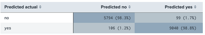
and where we see we are 98.3% accurate in predicting that a device does not have malware, and 98.8% accurate that it has.

So what?

We have a new Data & Cyber training programme coming up (supported by The Data Lab), and on 1 July 2020, you can find out about Machine Learning and Splunk. You can register here:

The course is presented over Zoom, and instructed led. It will teach you about all the different machine learning models, and how you analyse your data. All the course content will be delivered on-line, too, and with hands-on applications related to cybersecurity.

Background

In our data analysis for Cybersecurity we must often classify our data in order that we can efficiently search for things, or use it to trigger alerts from rules. A rule might relate to the blocking of access to a remote site. Thus our classification might relate to building up a list of whitelisted IP addresses and blacklisted ones. For each access, we may have to access the trustworthiness of an IP address, such as whether it is listed as malicious, or whether its domain name has existed for a specified amount of time. It we get it right, we have a successful classification, if it is wrong, then we have been unsuccessful. The success rate will then be defined as:

• True-positive (TP). That something has been successfully classified as the thing that we want it classified as.
• False-positive (FP). That we have classified something that is incorrect. This would be defined as a Type I error. An example might be where a system classifies an alert as a hack and where a user enters an incorrect password a number of times, but, on investigation, it is found that the valid user had just forgotten their password.
• True-negative (TN). That we rejected something, and it is not a match.
• False-negative (FN). That we have dismissed something, but, in fact, it is true. This is defined as a miss and is a Type II error. With this, a hacker might try a number of passwords for a user, and but where the system does not create an alert for the intrusion.

The Accuracy of the analysis could then be defined as:

Accuracy = (TP+TN)/total

The Sensitivity (or the True Positive Rate) is then the number of true positives (TP) against the number of times we have found a match (TP+FN):

Sensitivity = TP/(TP+FN)

The Sensitivity is also known as Recall.

Within Cybersecurity analytics, it is often the Sensitivity Rate which is seen to be a strong measure of the trustworthiness of the system. Thus the higher the Sensitivity rate, the higher the confidence that an analyst will have in the machine classification/search. If the Sensitivity Rate is low, the human analysts may lose trust in the machine to properly classify and find things correctly. A rate of 0.1, would mean that only one-in-ten classifications were actually correct. But this metric is not measuring the number of false positives, and these could confuse an analyst by investigating something that is not correct. So an improved measure might relate to the precision of the matches and will be the ratio of the true positive matches to the number of positive matches. In this example, we would have a precision of:

Precision = TP/(TP+FP)

In this case the analyst would have to deal with one in three false positives. For the Specificity we define the True Negative Rate, and when we do not have a match, how often do we predict it correctly? In our example, this we be:

Specificity = TN/(TN+FP)

And the False Positive Rate (FPR) is then 1 minus the Specificity. In our example, this we be:

False Positive Rate = FN/(TN+FN)

Prevalence then defines how often the system identifies something as being correct, as a ratio of all the data records that have been sampled. In our example, this we be:

Prevalence = (FN+TP)/Total

And so more …

Here’s more:

So what? Well, in partnership with The Data Lab, we are releasing a new MOOC on 3 August 2020, so watch this space. It will have a full Splunk learning environment, and where you can analyse a whole lot of cybersecurity data sets, and apply machine learning.