Introduction to Machine Learning and Splunk

Introduction to Machine Learning and Splunk — Predicting Categories

The future of cybersecurity is likely to see an increasing use of machine learning, and so that human analysts are not swamped by alerts. A core part of this is likely to be the usage of Splunk, and which plays an ever-increasing role in cybersecurity. We can use the machine learning infrastructure for predicting, forecasting and finding outliers. For these, we can either predict or forecast for numeric values (such as for integers or real values) or for categories (such as for different string values or yes/no).

Within forecasting, we might predict the failure of a hard disk, and when it is likely to happen, or the number of unsuccessful logins at a given time in the future. This forecasting allows us to make decisions before the time, and perhaps make interventions. For outliers, we also look at the normal band for the data and then filter to examine the ones that are outside this band. This could relate to the network traffic coming from an IoT device, and where we can find outliers that are sending more data than normal (as they could be infected with malware) or very little (as they may be faulty).

With prediction, we have a number of variables that we know about and use this to predict another value. For example, we might classify our data traffic with unencrypted data, encrypted data and Tor traffic. Based on small and constantly sized data packets for a given data stream, we might predict that we are data packets are using Tor. To make this prediction, we often need to show the machine learning model a range of different inputs and which are classified, and then the machine tries to find a model that fits the classification against the other parameters. If the value is a numerical value, such as the length of a data packet, we might be able to find a mathematical model that could calculate the value.

So let’s try an example:

Here is a dataset and a sample of the Python script that could be used:

After the Splunk Machine Learning App has been installed, we access it from the Apps interface, and then select the Splunk Machine Learning Toolkit:

Next, we create an Experiment from a number of options, such as for forecasting, outlier detection and prediction:

In this case, we will use a firewall log to predict that a device is infected by malware. Next, we give the experiment a name:

And then load up the data source (firewall_traffic.csv):

We can see it has over 98,000 records, so we can trim this down by just selecting the first 50,000 records:

Logistic Regression

In our machine learning model, we start with a dependent variable and have one or more predictor values (independent variables). These predictor values can either have two classes (a binary variable) or can be a real value (continuous value). In its normal form, the binary logistic model defines the probabilities that a data element will belong to one class or another. This may be yes/no, on/off, or pass/fail. With multimodal logistic regression, we can extend the method to have three or more classes for the dependent variable.

Basically, the method uses the log odds to determine probabilities. With log-odds, we take the chance of something happening and divide it by it not happening, and then take the natural log of that. For example, if we flip two coins, the chance of us getting two heads is one-in-four (0.25) and in not getting two heads is three-in-four (0.75). The log odds becomes ln(0.25/0.75) and which is -1.01.

So we can select a machine learning model of Logistic Regression and then select the field to train for “used_by_malware”:

After this, we can select the fields to be used to predict the field by selecting all the other fields. In this case, we then used 70% of the dataset to train and 30% of it to test our model against:

We then “Fit Model” and receive the results back from our data set:

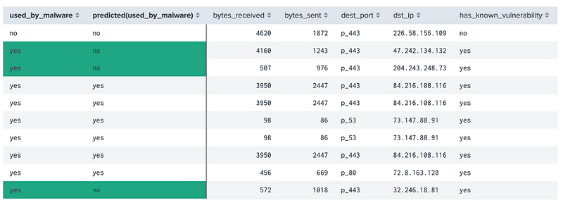
The highlighted values are incorrect. A predicted “yes” for a device not infected by malware is a false positive, and a predicted “yes” for a device which is infected is a true positive. Splunk automatically creates the evaluation metrics of Precision, Recall, Accuracy and F1, along with this confusion matrix:

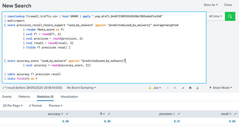
If we open up by clicking on the Confusion Matrix link, we see the script used:

If we select the “Open Search” on the button beside the “Build Model”, we get a script of:

We can make this look better by locating “|” and pressing SHIFT-ENTER to produce:

We can then paste in some code to do the same as the scoring table with the following:

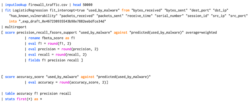
In this case, the square bracket ([]) is used to seed the output into two different inputs, and which gives:

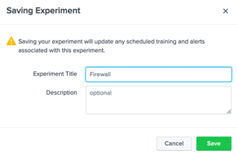
Finally we can save the experiment:

SVM

We will now use an SVM (Support Vector Machine) model and which is a supervised learning technique. Overall, it is used to create two categories and will try to allocate each of the training values into one category or the other. Basically, we have points in a multidimensional space and try to create a clear gap between the categories. New values are then placed within one of the two categories. In this case, we will train with SVM (see graphic on the left-hand side), and rerun the model. We now get a better model with:

Random Forest Linear Regression

With random forests we use a number of learning methods for classification and regression, and which involves the creation of many decision trees when training and then outlining a class to define the classification or mean prediction (regression) related to individual trees.

Using Random Forest Linear Regression, and get the best results:

Background

In our data analysis for Cybersecurity, we must often classify our data in order that we can efficiently search for things, or use it to trigger alerts from rules. A rule might relate to the blocking of access to a remote site. Thus our classification might relate to building up a list of whitelisted IP addresses and blacklisted ones. For each access, we may have to access the trustworthiness of an IP address, such as whether it is listed as malicious, or whether its domain name has existed for a specified amount of time. It we get it right, we have a successful classification, if it is wrong, then we have been unsuccessful. The success rate will then be defined as:

• True-positive (TP). That something has been successfully classified as the thing that we want it classified as.
• False-positive (FP). That we have classified something that is incorrect. This would be defined as a Type I error. An example might be where a system classifies an alert as a hack and where a user enters an incorrect password a number of times, but, on the investigation, it is found that the valid user had just forgotten their password.
• True-negative (TN). That we rejected something, and it is not a match.
• False-negative (FN). That we have dismissed something, but, in fact, it is true. This is defined as a miss and is a Type II error. With this, a hacker might try a number of passwords for a user, and but where the system does not create an alert for the intrusion.

The Accuracy of the analysis could then be defined as:

Accuracy = (TP+TN)/total

The Sensitivity (or the True Positive Rate) is then the number of true positives (TP) against the number of times we have found a match (TP+FN):

Sensitivity = TP/(TP+FN)

The Sensitivity is also known as Recall.

Within Cybersecurity analytics, it is often the Sensitivity Rate which is seen to be a strong measure of the trustworthiness of the system. Thus the higher the Sensitivity rate, the higher the confidence that an analyst will have in the machine classification/search. If the Sensitivity Rate is low, the human analysts may lose trust in the machine to properly classify and find things correctly.

A rate of 0.1, would mean that only one-in-ten classifications were actually correct. But this metric is not measuring the number of false positives, and these could confuse an analyst by investigating something that is not correct. So an improved measure might relate to the precision of the matches and will be the ratio of the true positive matches to the number of positive matches. In this example, we would have a precision of:

Precision = TP/(TP+FP)

In this case, the analyst would have to deal with one in three false positives. For the Specificity we define the True Negative Rate, and when we do not have a match, how often do we predict it correctly? In our example, this we be:

Specificity = TN/(TN+FP)

And the False Positive Rate (FPR) is then 1 minus the Specificity. In our example, this will be:

False Positive Rate = FN/(TN+FN)

Prevalence then defines how often the system identifies something as being correct, as a ratio of all the data records that have been sampled. In our example, this we be:

Prevalence = (FN+TP)/Total

So what?

We have a new online course here: