Cybersecurity and Machine Learning: Predicting Numeric Outliers

Cybersecurity and Machine Learning: Predicting Numeric Outliers

Cybersecurity is all about understanding normality

In the detection of Cybersecurity threats, we often need to understand what is normal, and what is not normal. This leads to either signature detection (detecting known things) and anomaly detection (detecting things that go away from the normal). For scripting type attacks, we often use a signature detection method, but in more human-focused attacks, we often focus on detecting when we move away from the normal. Someone who is committing fraud, for example, we often change their behaviour in some way. It is this change that could identify a possible threat.

For example, if the number of user logins at 9am on a Monday morning is normally 100 per hour, but then goes to 10 per hour, or 500 per hour, there might be a security issue (such users not being able to log in) or we may be under attack from a spear-phishing agent. It is thus important that we know what normal looks like, and then define boundaries for which our data move outside this.

Let’s start a new experiment with Splunk. For this we will detect a numeric outlier, so will select “Detect Numeric Outlier”:

And then a new experiment:

So let’s look at server response time, and understand the bounds of its operation. Overall, the hostperf.csv file [here] contains a timestamp for every second, processor limit, minimum response time, maximum response time, and average response time:

Next, we can then pick off the first 1,000 seconds, and then take the maximum value of the maximum response time as a 10-minute span:

| inputlookup hostperf.csv 
| eval _time=strptime(_time, “%Y-%m-%dT%H:%M:%S.%3Q%z”) 
| timechart span=10m max(rtmax) as responsetime 
| head 1000

This gives us a data set of which now has the maximum value within 10-minute slot:

2015–02–18 22:10:001.275
2015–02–18 22:20:005.933
2015–02–18 22:30:005.599
2015–02–18 22:40:002.839
2015–02–18 22:50:003.702
2015–02–18 23:00:004.602
2015–02–18 23:10:008.361
2015–02–18 23:20:0011.885
2015–02–18 23:30:005.519
2015–02–18 23:40:0010.044

We only have one field to analyse, so we can select the newly named field of responsetime:

Next, we need to look at how we define normality. For this we can determine the standard deviation for our data, or take the median absolute device, or even take the interquartile range:

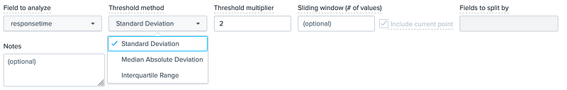
For the standard deviation method, we have an average (µ) and a standard deviation value (σ). The range of normality is then bounded by these values. We can also add a threshold multiplier, and which will often reduce the number of outliers, as we widen the normal range. If we now select the standard deviation method, we get 33 outliers:

Splunk then provides a chart of the daily outliers, and which shows the 19 Feb and 22 Feb were the days with the most outliers:

We can also view a distribution of the these within a band, and look at how the outliers move away from the mean:

If we now change for a multiplier of four, we see that our outliers drop to 6:

The great thing about Splunk is that you then end up with a script that can be easily integrated:

| inputlookup hostperf.csv 
| eval _time=strptime(_time, “%Y-%m-%dT%H:%M:%S.%3Q%z”) 
| timechart span=10m max(rtmax) as responsetime 
| head 1000

| eventstats avg(“responsetime”) as avg stdev(“responsetime”) as stdev 
| eval lowerBound=(avg-stdev*exact(4)), upperBound=(avg+stdev*exact(4))
| eval isOutlier=if(‘responsetime’ < lowerBound OR ‘responsetime’ > upperBound, 1, 0)

We can see we have functions related to avg() and stdev() to calculate the required parameters:

| eventstats avg(“responsetime”) as avg stdev(“responsetime”) as stdev

and then store these as the values of avg and stdev. Next, we calculate the lower bound and upper bound:

lowerBound=(avg-stdev*exact(4))
upperBound=(avg+stdev*exact(4))

We thus have µ- 4σ for the lower bound, and µ+4σ for the upper bound. Finally, we find the outliers with:

isOutlier=if(‘responsetime’ < lowerBound OR ‘responsetime’ > upperBound, 1, 0)

Once, we have our SPL (Search Programming Language) script, it’s an easy task to the modify the parameters. In this case we try a multiplier of two:

For the interquartile range we then split into quartiles, and where the 50th quartile defing the medium value (the value that splits the data set into 50/50). With percentiles we split the data into a number of ranges. With the 25th percentile, we have 25% of the data less than the 25th percentile point (p25), and with the 75th percentile, we have 75% of the data before the 75th percentile point (p75). With the interquartile range is the difference between p75 and p25, and thus have 50% of all the data. If we now add a multiplier of four, we have:

| eventstats median(“responsetime”) as median p25(“responsetime”) as p25 p75(“responsetime”) as p75 
| eval IQR=(p75-p25) 
| eval lowerBound=(median-IQR*exact(4)), upperBound=(median+IQR*exact(4))

For the medium absolute method, we determine the absolute value between the responsetime and the medium:

| eventstats median("responsetime") as median
| eval absDev=(abs(‘responsetime’-median)) 
| eventstats median(absDev) as medianAbsDev 
| eval lowerBound=(median-medianAbsDev*exact(4)), upperBound=(median+medianAbsDev*exact(4))

Conclusions

If you are interested, we will be releasing a new Cyber&Data programme, and supported by The Data Lab. Here is a forthcoming course: