Forcasting The Future With Splunk

Forecasting The Future With Splunk

Within any business, it is good to predict the future. How many people will buy ice cream when the temperatures hit 20C? How many users will log into our servers at 9am on a Monday morning. Luckily, data science comes to our rescue, and Splunk integrates with two well-defined methods for forecasting: Kalman Filter; and ARIMA:

With ARIMA (AutoRegressive Integrated Moving Average), we get a number of models, and which are stochastic (randomly generated) in their nature. Rather than defining a model, the Kalman filter is an algorithm and can be used to define a probability of the accuracy of the forecast. Kalman filters are often used in guidance systems, such as for navigation and the control of robots, aeroplanes, ships and spacecrafts. The human body can also be modeled with a Kalman filter for the way that our central nervous system controls our movements.

Overall we have a trend which defines the general change in a time series (such as an increase or decrease at a given rate over time). A seasonal element defines fluctuations for time, such as where ice cream sales will be largest in the July, and lowest in December. The logins to a network will also likely to have a seasonal component, as the weekend may show lower numbers of logins. The residual element is the background element of the data, when we take way the trend and seasonality.

In Splunk, we first create a “Forcast Time Series” experiment:

and then define a name for the experiment [here]:

We will use a trace of Internet traffic [here]:

| inputlookup internet_traffic.csv

This shows that the samples are taken in five minute intervals:

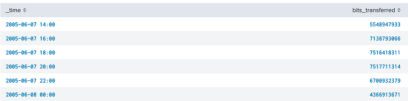
Now let’s group into two hour intervals, and create an average of bits transferred:

| inputlookup internet_traffic.csv 
| timechart span=120min avg(“bits_transferred”) as bits_transferred | eval bits_transferred=round(bits_transferred)

and which produces:

Now, let’s apply the Kalman Filter:

We can see that the Kalman Filter has a number of methods:

• LL (Local Level). Predict only local level of time series.
• LLT (Local Level Trend). Predict only trend.
• LLP (Seasonal Local Level). Predict only seasonal component;
• LLP5 (combines LLT and LLP). Predict with trend and seasonality.

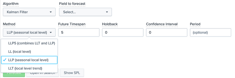
If we now use 100 future timestamps we get:

The SPL used for this is:

| inputlookup internet_traffic.csv 
| timechart span=120min avg(“bits_transferred”) as bits_transferred 
| eval bits_transferred=round(bits_transferred) 
| predict “bits_transferred” as prediction algorithm=LLP holdback=0 future_timespan=100 upper0=upper0 lower0=lower0 

The quality of the result is the R² statistic (the square of the coeffient), and where we aim to gain a value as near unity as possible. Now if we try LLP5, as we see an improvement in the R² statistic:

Bluetooth prediction

Now let’s use the data from a Bluetooth scanner, and try to predict the number of unique Bluetooth addresses that we expect to see over a given time period:

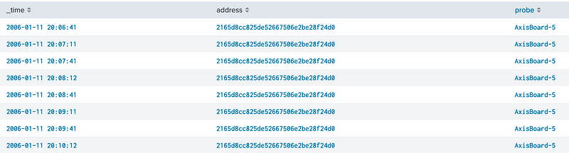
| inputlookup bluetooth.csv

This gives us a timestamped list of Bluetooth addresses, and the probe type [here]:

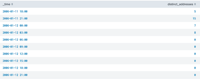
Now, we can then group them together, and define the number of unique addresses within a three hour period:

| inputlookup bluetooth.csv 
| where probe=”AxisBoard-5" 
| timechart dc(address) as distinct_addresses span=3h

and which shows five unique Bluetooth addresses from 6pm to 9pm, and then 15 addresses from 9pm to 12pm:

So let’s predict 100 time steps with a Malman Filter using the LLP method:

The result is then:

If we now try LLP5 we get an improved R² statistic:

Predicting logins

A typical task that we might have is to predicted the expected number of people who will login over a given time period. So let’s read-in a login dataset [here]:

| inputlookup login.csv

If we now predict, we get a good R² statistic:

Within the Kalman filter, we can also define a Holdback value, and which defines that we should not use the most recent values. We can then use the holdback values to detect how well we have predicted the forecast, In the following, we holdback for 50 time points, and then predict another 100 time points:

Conclusions

If you are interested, we will be releasing a new Cyber&Data programme, and supported by The Data Lab. Here is a forthcoming course: