The barriers to getting into machine learning have never been lower: Go do on ML

The barriers to getting into machine learning have never been lower: Go do ML

The need to code has never been so important. Why we don’t teach our kids to code at the earliest stage possible is beyond me?

The barrier to coding has never been so low. If you access repl.it, you can virtually ever programming language you want, and have it running in the Cloud. And now you can setup teams, where you can add as many students as you want. And it you want to get serious about your coding, you go and buy a R-PI, and you have a device which fits in your pocket and ready to code on.

The need to learn machine learning has never been higher. As a world we are increasingly swamped by data, and in areas such as cybersecurity, the need to process masses of data increases by the day.

The barrier to machline learning has never been lower. With Python, a machine learning programme can be created in minutes.

Go on …

So what’s holding you back? In this article, I will introduce the the key metrics used to define success in machine learning, and how we plot the ROC (Receiver Operating Characteristic).

And so here is the code:

• Code 1 (Show ROC (Receiver Operating Characteristic) Curve): [Here]
• Code 2 (Confusion Matrix for Handwriting numbers): [Here]
• Code 3 (Creating a data set with two clusters): [Here]
• Code 4 (Random Forest Classifier for numeric predictions with ROC curve and AUC (Area Under Curve): [Here]
• Code 5 (Numeric prediction with R2 metric): [Here]
• Code 6 (Numeric prediction and metrics): [Here]
• Code 7 (Category prediction and metrics): [Here]

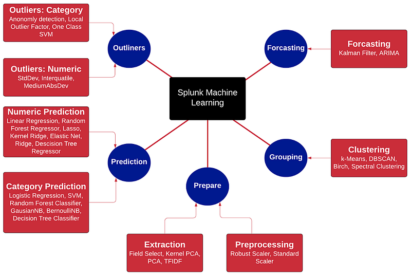
And here is how Splunk implements machine learning in the methods related to cybersecurity analysis:

Coding examples

Example Code 1: [Here]:

# https://asecuritysite.com/bigdata/roc
from sklearn import metrics
import matplotlib.pyplot as plt 

def show_roc(FPR, TPR, AUC):  
    plt.plot(FPR, TPR, color='blue', label='ROC')
    plt.plot([0, 1], [0, 1], color='darkblue', linestyle='--')
    plt.xlabel('FPR')
    plt.ylabel('TPR')
    plt.title('Receiver Operating Characteristic (ROC) Curve')
    plt.legend(["AUC=%.3f" % AUC])

    plt.show()

y = ['Eve', 'Eve', 'Eve', 'Eve','Eve','Bob','Bob', 'Bob','Bob','Bob']
scores = [20,25,16,42,22,50,41,60,54,39]

positive_label = 'Bob'

fpr, tpr, thresholds = metrics.roc_curve(y, scores, pos_label=positive_label)

auc=metrics.auc(fpr, tpr)

print ("FPR:",fpr)
print ("TPR:",tpr)

print ("Thresholds:",thresholds)

show_roc(fpr, tpr,auc)

Example Code 2 [Here]

# https://asecuritysite.com/bigdata/sk01
import sys
import matplotlib.pyplot as plt

ga=0.011

if (len(sys.argv)>1):
	file=str(sys.argv[1])

if (len(sys.argv)>2):
	ga=float(sys.argv[2])

from sklearn import datasets, svm, metrics

digits = datasets.load_digits()

images_and_labels = list(zip(digits.images, digits.target))
for index, (image, label) in enumerate(images_and_labels[:10]):
    plt.subplot(2, 10, (index + 1))
    plt.axis('off')
    plt.imshow(image, cmap=plt.cm.gray_r, interpolation='nearest')
    plt.title('Tr: %i' % label)

# To apply a classifier on this data, we need to flatten the image, to
# turn the data in a (samples, feature) matrix:
n_samples = len(digits.images)
data = digits.images.reshape((n_samples, -1))

# Create a classifier: a support vector classifier
classifier = svm.SVC(gamma=ga)

# We learn the digits on the first half of the digits
classifier.fit(data[:n_samples // 2], digits.target[:n_samples // 2])

# Now predict the value of the digit on the second half:
expected = digits.target[n_samples // 2:]
predicted = classifier.predict(data[n_samples // 2:])

print("Classification report for classifier %s:\n%s\n"
      % (classifier, metrics.classification_report(expected, predicted)))
print("Confusion matrix:\n%s" % metrics.confusion_matrix(expected, predicted))

images_and_predictions = list(zip(digits.images[n_samples // 2:], predicted))
for index, (image, prediction) in enumerate(images_and_predictions[:4]):
    plt.subplot(2, 4, index + 5)
    plt.axis('off')
    plt.imshow(image, cmap=plt.cm.gray_r, interpolation='nearest')
    plt.title('Prediction: %i' % prediction)

plt.show()

Example Code 3: [Here]

# This code creates a data set with two clusters (defined by the two features. The output is then data_vals[:, 0] and data_vals[:, 1] and these are marked by class_lab

from sklearn.datasets import make_classification  
import matplotlib.pyplot as plt 

data_vals, class_label =make_classification(n_samples=100,n_features=2, n_redundant=0, n_informative=1,n_clusters_per_class=1)

plt.scatter(data_vals[:, 0], data_vals[:, 1], marker='o', c=class_label,s=25, edgecolor='k')

plt.savefig('test.png')

plt.show()

Example Code 4: [Here]

# Create ROC 
from sklearn.datasets import make_classification  
from sklearn.model_selection import train_test_split 
from sklearn.ensemble import RandomForestClassifier
from sklearn.metrics import roc_auc_score 
from sklearn.metrics import roc_curve 
import matplotlib.pyplot as plt 

def show_roc(FPR, TPR, AUC):  
    plt.plot(FPR, TPR, color='blue', label='ROC')
    plt.plot([0, 1], [0, 1], color='darkblue', linestyle='--')
    plt.xlabel('FPR')
    plt.ylabel('TPR')
    plt.title('Receiver Operating Characteristic (ROC) Curve')
    plt.legend(["AUC=%.3f" % AUC])
    plt.show()

data_vals, class_label =make_classification(n_samples=100,n_features=2, n_redundant=0, n_informative=1,n_clusters_per_class=1)

X_train, X_test, y_train, y_test = train_test_split(data_vals, class_label, test_size=0.3, random_state=1) 

# RandomForestClassifier, BaggingClassifier, ExtraTreesClassifier, AdaBoostClassifier, and GradientBoostingRegressor.
model = RandomForestClassifier() 

model.fit(X_train, y_train)  

y_predict = model.predict_proba(X_test) 

print ("Model score: ",model.score(X_test, y_test))

# probablities of getting a 1
y_predict = y_predict[:, 1]  

auc = roc_auc_score(y_test, y_predict)  

FPR, TPR, thresholds = roc_curve(y_test, y_predict) 

print ("Thresholds: ",thresholds)
print ("FPR: ",FPR)
print ("TPR: ",TPR)

show_roc(FPR, TPR,auc) 

plt.scatter(data_vals[:, 0], data_vals[:, 1], marker='o', c=class_label,s=25, edgecolor='k')

plt.savefig('test.png')

Code sample 5: [Here]

from sklearn.metrics import r2_score, mean_squared_error,max_error,mean_squared_log_error
bob_login = [48, 12, 7, 11,43,44]
bob_predicted= [41, 14, 9, 15,40,41]

print ("R^2 score: ",r2_score(bob_login, bob_predicted))
print ("RMSE score: ",mean_squared_error(bob_login, bob_predicted))
print ("Mean squared error: ",mean_squared_log_error(bob_login, bob_predicted))

print ("Max error: ",max_error(bob_login, bob_predicted))

Code 6 (Numeric Prediction): [Here]

import pandas as pd
from sklearn.model_selection import train_test_split
from sklearn.ensemble import RandomForestRegressor
from sklearn.metrics import r2_score,mean_squared_error

# Features
x1= "blood_pressure"
x2= "age"
# Prediction
x3 = "BMI"

fdata="diabetes.csv"

print ("Training data:\t\t",x1,",",x2)
print ("Training against:\t",x3)
print ("Data set:\t\t",fdata)

ver=pd.read_csv(fdata)

dataset=ver[[x1,x2]]
train=ver[x3]
print (dataset)

x_train, x_test, y_train, y_test= train_test_split(dataset,train,test_size=0.3, random_state=1)

model= RandomForestRegressor()

model.fit(x_train,y_train)

y_predictions =model.predict(x_test)

accuracy = r2_score(y_test, y_predictions)
mse = mean_squared_error(y_test, y_predictions)

print ("R^2=",accuracy)
print ("MSE=",mse)

Code 7 (Cluster prediction and metrics): [Here]

# Cluster Prediction 
import pandas as pd
from sklearn.model_selection import train_test_split
from sklearn.cluster import KMeans
from sklearn.metrics import confusion_matrix, roc_curve, auc

# Features
x1= "blood_pressure"
x2= "age"
# Prediction
x3 = "response"

fdata="diabetes.csv"

print ("Training data:\t\t",x1,",",x2)
print ("Training against:\t",x3)
print ("Data set:\t\t",fdata)

ver=pd.read_csv(fdata)

dataset=ver[[x1,x2]]
train=ver[x3]
print (dataset)

x_train, x_test, y_train, y_test= train_test_split(dataset,train,test_size=0.3, random_state=1)

model=  KMeans(n_clusters=2, random_state=0)

model.fit(x_train,y_train)

y_predictions =model.predict(x_test)

conf=confusion_matrix(y_test,y_predictions)
print (conf)

fpr, tpr, thresholds = roc_curve(y_test,y_predictions)

auc=auc(fpr, tpr)

print ("FPR:",fpr)
print ("TPR:",tpr)

print ("Thresholds:",thresholds)

print ("AUC: ",auc)

Tutorial

1. We want to differentiate Eve from Bob. In monitoring Eve’s accesses to email on a daily basis we find daily accesses of 20, 25, 16, 42 and 22, and then monitory Bob’s accesses as: 50, 41, 60, 54 and 39. With the following we aim to detect Bob from Eve, and plot the ROC Curve. Use the following code to determine the ROC curve and the AUC value:

htps://repl.it/@billbuchanan/class01

Listing:

# https://asecuritysite.com/bigdata/roc
from sklearn import metrics
import matplotlib.pyplot as plt

def show_roc(FPR, TPR, AUC):
plt.plot(FPR, TPR, color='blue', label='ROC')
plt.plot([0, 1], [0, 1], color='darkblue', linestyle='--')
plt.xlabel('FPR')
plt.ylabel('TPR')
plt.title('Receiver Operating Characteristic (ROC) Curve')
plt.legend(["AUC=%.3f" % AUC])

plt.show()

y = ['Eve', 'Eve', 'Eve', 'Eve','Eve','Bob','Bob', 'Bob','Bob','Bob']
scores = [20,25,16,42,22,50,41,60,54,39]

positive_label = 'Bob'

fpr, tpr, thresholds = metrics.roc_curve(y, scores, pos_label=positive_label)

auc=metrics.auc(fpr, tpr)

print ("FPR:",fpr)
print ("TPR:",tpr)

print ("Thresholds:",thresholds)

show_roc(fpr, tpr,auc)

What is the AUC:

What are the thresholds used?

For each threshold, what is the FPR and what is the TPR:

If we set a threshold of 42, what is the FPR and what is the TPR?

Bob’s daily accesses for email are now monitored for 50, 55, 43, 90, 110 and 66, and Eve has accesses of 14, 32, 19, 46, 21, 48 and 50. Use the program to determine the new ROC curve:

What is the AUC:

What are the thresholds used?

For each threshold, what is the FPR and what is the TPR:

If we set a threshold of 42, what is the FPR and what is the TPR?

2. Now, we can add Alice, and who has accesses of 13, 23, 32, 40, 11, and 14, and determine the following:

What is the AUC:
 What are the thresholds used?
 For each threshold, what is the FPR and what is the TPR:
 If we set a threshold of 42, what is the FPR and what is the TPR?

3. Now change the positive label to Alice, and determine the following:

What is the AUC:

What are the thresholds used?

For each threshold, what is the FPR and what is the TPR:

If we set a threshold of 42, what is the FPR and what is the TPR?

In the following example we will load a dataset for a machine learning model to differentiate hand written digits. Run the following code and determine the confusion matrix:

htps://repl.it/@billbuchanan/class02

# https://asecuritysite.com/bigdata/sk01
import sys
import matplotlib.pyplot as plt

ga=0.011

from sklearn import datasets, svm, metrics

digits = datasets.load_digits()

images_and_labels = list(zip(digits.images, digits.target))
for index, (image, label) in enumerate(images_and_labels[:10]):
plt.subplot(2, 10, (index + 1))
plt.axis('off')
plt.imshow(image, cmap=plt.cm.gray_r, interpolation='nearest')
plt.title('Tr: %i' % label)

# To apply a classifier on this data, we need to flatten the image, to
# turn the data in a (samples, feature) matrix:
n_samples = len(digits.images)
data = digits.images.reshape((n_samples, -1))

# Create a classifier: a support vector classifier
classifier = svm.SVC(gamma=ga)

# We learn the digits on the first half of the digits
classifier.fit(data[:n_samples // 2], digits.target[:n_samples // 2])

# Now predict the value of the digit on the second half:
expected = digits.target[n_samples // 2:]
predicted = classifier.predict(data[n_samples // 2:])

print("Classification report for classifier %s:\n%s\n"
% (classifier, metrics.classification_report(expected, predicted)))
print("Confusion matrix:\n%s" % metrics.confusion_matrix(expected, predicted))

images_and_predictions = list(zip(digits.images[n_samples // 2:], predicted))
for index, (image, prediction) in enumerate(images_and_predictions[:4]):
plt.subplot(2, 4, index + 5)
plt.axis('off')
plt.imshow(image, cmap=plt.cm.gray_r, interpolation='nearest')
plt.title('Prediction: %i' % prediction)

plt.show()

What are the TP for the character ‘0’

What are the FP for the character ‘0’

What are the FP for the character ‘0’

We are using SVM (Support Vector Machine), and which uses a gamma factor. Vary the gamma value with 0.1, 0.2, 0.3 and so on, up to 1.0, and observe how the confusion matrix changes:

5. The following code generates a data set which has two clusters, and then marks each of the dataset elements for their cluster source. Run the program several times and observe the creation of the clusters:

htps://repl.it/@billbuchanan/class03

# This code creates a data set with two clusters (defined by the two features. The output is then data_vals[:, 0] and data_vals[:, 1] and these are marked by class_lab

from sklearn.datasets import make_classification
import matplotlib.pyplot as plt

data_vals, class_label =make_classification(n_samples=100,n_features=2, n_redundant=0, n_informative=1,n_clusters_per_class=1)

plt.scatter(data_vals[:, 0], data_vals[:, 1], marker='o', c=class_label,s=25, edgecolor='k')

plt.savefig('test.png')

plt.show()

Modify the code so that it now generates 250 points.

6. We will now use this method of cluster generation, and then split the data into 70% training data, and 30% test data, in to train a RandomForestClassifier model to predict the results:

htps://repl.it/@billbuchanan/class04

# Create ROC
from sklearn.datasets import make_classification
from sklearn.model_selection import train_test_split
from sklearn.ensemble import RandomForestClassifier
from sklearn.metrics import roc_auc_score
from sklearn.metrics import roc_curve
import matplotlib.pyplot as plt

def show_roc(FPR, TPR, AUC):
plt.plot(FPR, TPR, color='blue', label='ROC')
plt.plot([0, 1], [0, 1], color='darkblue', linestyle='--')
plt.xlabel('FPR')
plt.ylabel('TPR')
plt.title('Receiver Operating Characteristic (ROC) Curve')
plt.legend(["AUC=%.3f" % AUC])
plt.show()

data_vals, class_label =make_classification(n_samples=10,n_features=2, n_redundant=0, n_informative=1,n_clusters_per_class=1)

X_train, X_test, y_train, y_test = train_test_split(data_vals, class_label, test_size=0.3, random_state=1)

model = RandomForestClassifier()

model.fit(X_train, y_train)
print ("Model score: ",model.score(X_test, y_test))

probs = model.predict_proba(X_test)

# probabilities of getting a 1
probs = probs[:, 1]

auc = roc_auc_score(y_test, probs)

FPR, TPR, thresholds = roc_curve(y_test, probs)

print ("Thresholds: ",thresholds)
print ("FPR: ",FPR)
print ("TPR: ",TPR)

show_roc(FPR, TPR,auc)

plt.scatter(data_vals[:, 0], data_vals[:, 1], marker='o', c=class_label,s=25, edgecolor='k')

plt.savefig('test.png')

For 10 points, what is the AUC?
 For 100 points, what is the AUC?
 For 250 points, what is the AUC?
 For 1000 points, what is the AUC?
 For the different number of points, how does the shape of ROC Curve change?

7. There are a few ensemble methods for machine learning in skLearn, including BaggingClassifier, ExtraTreesClassifier, AdaBoostClassifier, and GradientBoostingRegressor. Modify the code given in Q.6 to support each of the different models:

from sklearn.ensemble import AdaBoostClassifier
...
model = AdaBoostClassifier()

For each of the methods, what is the AUC, and which method is the best performing? ExtraTreesClassifier AUC: AdaBoostClassifier AUC: GradientBoostingRegressor AUC: BaggingClassifier AUC:

8. You have been asked to identify if there is a linkage between gun ownership and population density in US states, and whether there is a link to the number of murders per 100K of the population. An outline of the code is given here:

htps://repl.it/@billbuchanan/class08

# Numeric Prediction
import pandas as pd
from sklearn.model_selection import train_test_split
from sklearn.ensemble import RandomForestRegressor
from sklearn.metrics import r2_score,mean_squared_error

# Features
x1= "Gun ownership"
x2= "Population density"
# Prediction
x3 = "Murders per 100K"

fdata="guns.csv"

print ("Training data:\t\t",x1,",",x2)
print ("Training against:\t",x3)
print ("Data set:\t\t",fdata)

ver=pd.read_csv(fdata)

dataset=ver[[x1,x2]]
train=ver[x3]
print (dataset)

x_train, x_test, y_train, y_test= train_test_split(dataset,train,test_size=0.3, random_state=1)

model= RandomForestRegressor()

model.fit(x_train,y_train)

y_predictions =model.predict(x_test)

accuracy = r2_score(y_test, y_predictions)
mse = mean_squared_error(y_test, y_predictions)

print ("R^2=",accuracy)
print ("MSE=",mse)

# Correlation
cor=ver.corr()
print (cor[x3])

By examining the R2 value, is the machine learning implementation a good model?

Can you create a better model for predicting Murders per 100K pf the population, and with only two features?

Conclusions

We have a new MSc in the planning related to Cyber&Data, here’s a little taster:

https://asecuritysite.com/cyberdata