Breaking A (Crypto) Rainbow

Breaking A (Crypto) Rainbow

And, so, in the next decade or so we will see a move away from our existing public key methods of RSA and ECC and towards quantum robust methods. But, one contenders for the digital signature standard has perhaps fallen at the first fence. For this, Ward Beullens has just published [here] a paper that breaks Rainbow in less than a weekend:

Rainbow was never likely to win, as it struggles in most areas against the other two lattice methods:

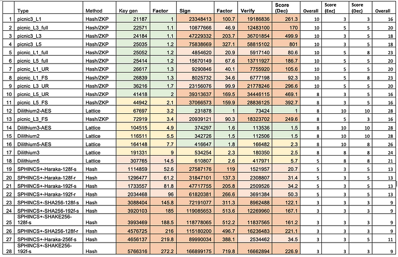
The other two finalists are Falcon and Dilithium, and which are so much faster for generation, signing and verifying. But, it is a surprise that Rainbow managed to get to the final, and for this new crack to have not been investigated before. The Sage implementation of the crack is here, and took around 50 hours on an eight core laptop.

Oil and Vineger

Overall, quantum computers will be able to break our existing public key methods, such as discrete logs, RSA and elliptic curve. And so NIST has created a Post Quantum Cryptography competition, and one of the methods is known as Rainbow. This is known as the Oil and Vinegar method and uses multivariate cryptography with an added trapdoor. So let’s take a simple example, and work through how the trapdoor works.

With multivariate cryptography, we have n variables within polynomial equations. For example, if we have four variables (w,x,y,z) and an order of two, we could have [here]:

w²+4wx+3x²+2wy−4wz+2wx+6xz=387

Generally, this is a hard problem to solve, so we want to make it easy if we know a secret. In this case, I know that the solution is w=7,x=4,y=5, and z=6. For a matrix form, we could represent this as:

This matrix has a trapdoor, and where we define our vinegar and oil variables. The vinegar variables are secret and which we will only know, and the oil ones will be discovered if we know the vinegar variables. The trap door is that we do not let the oil variables mix, and where they do mix in the matrix we will have zeros (the trap door):

In order to contain the values we get, we normally perform (mod p) operation and where p is a prime number. This is known as a finite field, and are numbers are always constrained between 0 and p−1. For example, if we select p=97 we have:

w²+4wx+3x²+2wy−4wz+2wx+6xz=5 (mod 97)

Now there are multiple solutions to this now for w,x,y,z, so we define n multivariate polynomials. For example:

w²+4wx+3x²+2wy−4xz+2wx+6xy=96 (mod 97)

5w²+3wx+3x²+4wy−xz+8wx+4xy=36 (mod 97)

4w²+5wx+3x²+2wy−5xz+3wx+6xy=95 (mod 97)

6w²+7wx+4x²+2wy−8xz+2wx+9xy=17 (mod 97)

With large values of the variables, this is a known hard problem to solve. So now we define our vinegar variables of w and x and oil variables of y and z. If we know w and x it will now become easy to determine oil variables. For example, if w=7 and x=4, we get:

49+112+48+14y−16z+14z+24y=96 (mod 97)

245+84+48+28y−4z+56z+16y=36 (mod 97)

and gives:

209+38y−2z=96 (mod 97)

377+44y+52z=36 (mod 97)

and gives:

38y+95z=−113 (mod 97)

44y+52z=−341 (mod 97)

and gives:

38y+95z=81 (mod 97)

44y+52z=47 (mod 97)

This is now a simple linear equation (in a modulo form), and which can be easily solved. In a matrix form this becomes:

and we can solve for y and z with:

We can now easily solve this with y=5 and z=6. Here is the code [here]:

import numpy as np
from inv import modMatInv
import sys

p=97

w=7
x=4

if (len(sys.argv)>1):
    w=int(sys.argv[1])
if (len(sys.argv)>2):
    x=int(sys.argv[2])

if (len(sys.argv)>3):
    p=int(sys.argv[3])

def printM(M):
  rtn = ""+str(M[0][0])+"w^2 + "+str(M[0][1]+M[1][0])+"wx + "+str(M[1][1])+"x^2 + "+str(M[0][2]+M[2][0])+"wy + "+str(M[1][3]+M[3][1])+"xz + " +str(M[0][3]+M[3][0])+"wz + "+str(M[1][2]+M[2][1])+"xy" 
  return rtn

def revealM(M,w,x):
  rtn = ""+str(M[0][0]*w*w) +" + "+str((M[0][1]+M[1][0])*w*x)+" + "+str(M[1][1]*x*x)+" + "+str((M[0][2]+M[2][0])*w)+"y + "+str((M[1][3]+M[3][1])*x)+"z + " +str((M[0][3]+M[3][0])*w)+"z + "+str((M[1][2]+M[2][1])*x)+"y" 
  return rtn

M0=[[1,2,1,1],[2,3,3,-2],[1,3,0,0],[1,-2,0,0]]
M1=[[5,2,1,2],[1,3,2,2],[3,2,0,0],[6,-3,0,0]]
M2=[[4,2,2,1],[3,3,3,-2],[0,3,0,0],[2,-3,0,0]]
M3=[[6,2,1,1],[5,4,3,-3],[1,6,0,0],[1,-5,0,0]]

print ("p=",p)

print ("\nM0:",M0)
print ("M1:",M1)
print ("M2:",M2)
print ("M3:",M3)

# res = m . M0 . m^{-1}
res0=96
res1=36
res2=95
res3=17

a=(res0-(M0[0][0]*(w*w)+(M0[0][1]+M0[1][0])*w*x + (M0[1][1])*x*x ) ) %p
b=(res1-(M1[0][0]*(w*w)+(M1[0][1]+M1[1][0])*w*x + (M1[1][1])*x*x ) ) %p

factor1=( ((M0[0][2]+M0[2][0])*w) +  ((M0[1][2]+M0[2][1]) *x) )  %p
factor2=( ((M0[0][3]+M0[3][0])*w) + ((M0[1][3]+M0[3][1]) *x) )  %p
factor3=( (M1[0][2]+M1[2][0])*w) +  ((M1[1][2]+M1[2][1]) *x)  %p
factor4=( ((M1[0][3]+M1[3][0])*w) + ((M1[1][3]+M1[3][1])*x))  %p

print ("w=",w)
print ("x=",x)
print (printM(M0))
print (printM(M1))
print ()
print (revealM(M0,w,x))
print (revealM(M1,w,x))
print ()
print (str(factor1)+"y+"+str(factor2)+"z="+str(a))
print (str(factor3)+"y+"+str(factor4)+"z="+str(b))
print ()

A = np.array([[factor1,factor2], [factor3,factor4]])
B = np.array([a,b])

invA = modMatInv(A,p)

print (invA)

res = np.dot(invA,B) % p

print ("y=",res[0])
print ("z=",res[1])

And a sample run [here]:

p= 97

M0: [[1, 2, 1, 1], [2, 3, 3, -2], [1, 3, 0, 0], [1, -2, 0, 0]]
M1: [[5, 2, 1, 2], [1, 3, 2, 2], [3, 2, 0, 0], [6, -3, 0, 0]]
M2: [[4, 2, 2, 1], [3, 3, 3, -2], [0, 3, 0, 0], [2, -3, 0, 0]]
M3: [[6, 2, 1, 1], [5, 4, 3, -3], [1, 6, 0, 0], [1, -5, 0, 0]]
w= 7
x= 4
1w^2 + 4wx + 3x^2 + 2wy + -4xz + 2wz + 6xy
5w^2 + 3wx + 3x^2 + 4wy + -1xz + 8wz + 4xy

49 + 112 + 48 + 14y + -16z + 14z + 24y
245 + 84 + 48 + 28y + -4z + 56z + 16y

38y+95z=81
44y+52z=47

Inverse matrix:
 [[63. 36.]
 [81.  5.]]
y= 5.0
z= 6.0

Here is the full code:

https://replit.com/@billbuchanan/ov

Conclusions

Not a great sign, but hopefully the lattice methods will provide a stronger foundation.