So What’s A Modulus In Post Quantum Cryptography?

So What’s A Modulus In Post Quantum Cryptography?

If you are into cybersecurity or secure software development, you may have learned about public key encryption and of the methods that were created around the end of the 1970s and in the 1980s. Well, you may just have to learn some more theory — as the methods you learnt could be under threat from quantum computers.

So, if you want to start you learning about these new methods, then read on. If you are happy to live in a pre-post quantum world of public key encryption, then perhaps stop reading.

The (mod p) operation

In traditional public key encryption, we use a modulus to create a finite field. While it might sound complex, it actually quite a simple concept. For a finite field, we introduce a modulus, and which is normally a prime number. So with the prime number we basically determine the remainder from an integer divide, and then take the remainder as the result. For example, if we have a prime number of 17, we will have output values that range from 0 to 16:

5 (mod 17) = 6
19 (mod 17) = 2
100 (mod 17) = 15

The great thing with the (mod p) operation, is that we can still add, subtract, multiply and divide, and end up with the same result, such as:

15 (mod 17) + 100 (mod 17) = (15+100) (mod 17) = 13
15 (mod 17) * 100 (mod 17) = (15*100) (mod 17) = 4

In discrete logs, we often use the Diffie Hellman method, and where we select a shared prime number (p) and a shared generator value (g), and compute:

A = g^x (mod p)
B = g^y (mod p)

A and B are exchanged, and the shared key is then:

K = A^y (mod p)

The works because:

K = A^y (mod p) = (g^x)^y (mod p) = g^{x.y} (mod p)

In the RSA method, we use a modulus (N). For ciphering, we have:

C = M^e (mod N)

and to decipher:

M = C^d (mod N)

In this case, N is the multiplication of two prime numbers, and the strength of RSA lies in the difficulty of factorizing the modulus (N). Elliptic curve methods, too, use a modulus of a prime number (p), and where we have:

y² =x³ + a.x + b (mod p)

This constrains the values of the points we use on the elliptic curve between 0 and (p-1).

Polynomials

But, quantum computers will break RSA, elliptic curves and discrete logs, so what is the equivalent to the modulus in post-quantum cryptography? Well, with this we can use lattice cryptography, and which involves us using polynomial values to represent our bit strings.

If we have a value of 19, it can be represented as 10011 and as a polynomial value of:

x⁴+x+1

and 67 can be represented by 1000011 and as a polynomial:

x⁶+x+1

If we add the two polynomials, we get:

(x⁴+x+1)+(x⁶+x+1)=x⁶+x⁴+1+1

And because we are using Base 2, 1+1 is equal to 0, thus we get:

(x⁴+x+1)+(x⁶+x+1)=x⁶+x⁴

The same goes for adding the same power, such as:

x⁴ + x⁴ = 0
x⁴ + x⁴ + x⁴ = x⁴
and so on.

And, so, in lattice cryptography we add, subtract, multiply and divide by polynomials. An operation may have a polynomial value of x³+x+1, and then a secret polynomial of x²+1, and might multiply them to get a result. To recover the value back again, we can then just divide by the secret polynomial.

But, how do we constrain the maximum power of the polynomial within a finite field? Well for this — as we did with our traditional public key methods — we use a modulus, and where we divide by the modulus and keep the remainder.

Modulus in Galois Fields

A finite field or Galois field (GF) has a finite number of elements and has an order which is equal to a prime number (GF(p)) or to the power of a prime number (GF(2^p)). For example, GF(2^n) has 2^n elements, and its elements are known as binary polynomials (where the coefficients of the polynomial factors either are either zero or one value. In order to reduce a polynomial to a given size, we use a modulus polynomial, and which divides the output value. For GF(128), we can use a modulus of x⁷+x+1.

So let’s take an example:

a=x³+x²+1

b=x⁶+x⁴+x³+1

When we add, we get:

a+b=x³+x²+1+x⁶+x⁴+x³+1=x⁶+x⁴+x²

Now, let’s multiply them:

a×b=(x³+x²+1)×(x⁶+x⁴+x³+1)=x⁹+x⁷+x⁶+x³+x⁸+x⁶+x⁵+x²+x⁶+x⁴+x³+1=x⁹+x⁸+x⁷+x⁵+x⁴+x²+1

We now divide this value by the modulus. In this case for GF(128), the modulus is x⁷+x+1:

              x^2 + x + 1
            -------------------------------------------------------
x^7 + x + 1 | x^9 + x^8 + x^7 + x^6 + x^5 + x^4 +      x^2 +      1
              x^9 +                               x^3 +x^2
                    -----------------------------------------------
                    x^8 + x^7 + x^6 + x^5 + x^4 + x^3      +      1
                    x^8                               +x^2 + x
                    -----------------------------------------------
                          x^7 + x^6 + x^5 + x^4 + x^3 + x^2 + x + 1
                          x^7                               + x + 1
                    -----------------------------------------------
                               x^6 + x^5 + x^4 + x^3 + x^2

For GF(128), the result of a×b is thus:

a×b=x⁶+x⁵+x⁴+x³+x²

In Sage, we can code this with [here]:

print (f"GF: {GF(128)}")
F. = GF(128)
print (f"Modulus = {F.modulus()}")
a = x^3+ x^2 + 1
b = x^6 + x^4+ x^3 + 1
print (f"a = {a}")
print (f"b = {b}")
print (f"a - b = {a - b}")
print (f"a + b = {a + b}")
print (f"a * b = {a * b}")
print (f"a / b = {a / b}")
print (f"a^-1 =  {a^-1}")
print (f"1/b =  {1/b}")

And a sample run is [here]:

a = x^3 + x^2 + 1
b = x^6 + x^4 + x^3 + 1
Modulus = x^7 + x + 1
a - b = x^6 + x^4 + x^2
a + b = x^6 + x^4 + x^2
a * b = x^6 + x^5 + x^4 + x^3 + x^2
a / b = x^4
a^-1 =  x^6 + x^3 + x^2 + x + 1
1/b =  x^6 + x^5 + x^3 + x + 1

If we now use GF(256) [here]:

print (f"GF: {GF(256)}")
F. = GF(256)
print (f"Modulus = {F.modulus()}")
a = x^3+ x^2 + 1
b = x^6 + x^4+ x^3 + 1
print (f"a = {a}")
print (f"b = {b}")
print (f"a - b = {a - b}")
print (f"a + b = {a + b}")
print (f"a * b = {a * b}")
print (f"a / b = {a / b}")
print (f"a^-1 =  {a^-1}")
print (f"1/b =  {1/b}")

A sample run is [here]:

GF: Finite Field in z7 of size 2^7
Modulus = x^8 + x^4 + x^3 + x^2 + 1
a = x^3 + x^2 + 1
b = x^6 + x^4 + x^3 + 1
a - b = x^6 + x^4 + x^2
a + b = x^6 + x^4 + x^2
a * b = x^7 + x^6 + x^4 + x
a / b = x^7 + x^5 + x^2
a^-1 =  x^7 + x^5 + x^3 + x
1/b =  x^7 + x^6 + 1

We can see that the default modulus of GF(256) in Sage is then:

x⁸+x⁴+x³+x²+1

We can list the default modulus values in Sage with [here]:

F. = GF(2)
print (f"GF(2) Modulus = {F.modulus()}")
F. = GF(4)
print (f"GF(4) Modulus = {F.modulus()}")
F. = GF(8)
print (f"GF(8) Modulus = {F.modulus()}")
F. = GF(16)
print (f"GF(16) Modulus = {F.modulus()}")
F. = GF(32)
print (f"GF(32) Modulus = {F.modulus()}")
F. = GF(64)
print (f"GF(64) Modulus = {F.modulus()}")
F. = GF(128)
print (f"GF(128) Modulus = {F.modulus()}")
F. = GF(256)
print (f"GF(256) Modulus = {F.modulus()}")
F. = GF(512)
print (f"GF(512) Modulus = {F.modulus()}")

This gives [here]:

GF(2) Modulus = x + 1
GF(4) Modulus = x^2 + x + 1
GF(8) Modulus = x^3 + x + 1
GF(16) Modulus = x^4 + x + 1
GF(32) Modulus = x^5 + x^2 + 1
GF(64) Modulus = x^6 + x^4 + x^3 + x + 1
GF(128) Modulus = x^7 + x + 1
GF(256) Modulus = x^8 + x^4 + x^3 + x^2 + 1
GF(512) Modulus = x^9 + x^4 + 1

Irreducible polynomial

Just like our prime number in public key encryption, we need a polynomial that cannot be divided by anything. For this, we use an irreducible polynomial. Examples of irreducible polynomials are [here]:

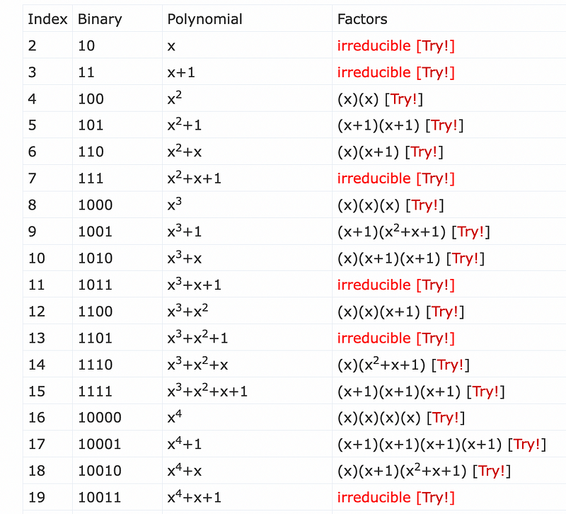
Our irreducible polynomials are the x, x², x²+x+1, and x³+x²+1. These are equivalent to the prime numbers we use in our traditional public key encryption methods, and are similar to the (mod p) operation. A popular one is x⁸+x⁴+x³+x+1, and which is used in AES encryption. In Sage, we can define our own modulus, such as:

k.<x>= GF(2^8, modulus=x^8+x^4+x^3+x+1)

If we have an input value 101101 of y=x⁵+x³+x²+1, and we multiply by h=x⁴+x+1, we get:

r = y.h = (x⁵+x³+x²+1) × (x⁴+x+1)

We can then create the following Sage code [here]:

# Rijndael finite field
k.<x>= GF(2^8, modulus=x^8+x^4+x^3+x+1)
y = (x^5+x^3+x^2+1)
h= (x^4+x+1)
r=y*h
print(f"(x^5+x^3+x^2+1) * (x^4+x+1)= {r} ({r.integer_representation()})")

When we run we get the result of [here]:

$ sage 1.sage
(x^5+x^3+x^2+1) * (x^4+x+1)= x^7 + x^4 + 1 (145)

Now we can divide by our irreducible polynomial and get the original value back again [here]:

# Rijndael finite field
k.<x>= GF(2^8, modulus=x^8+x^4+x^3+x+1)
y = (x^5+x^3+x^2+1)
h= (x^4+x+1)
r=y*h
r2=r/h
print(f"{r}/ (x^4+x+1)= {r2} ({r2.integer_representation()})")

and get the result of [here]:

$ sage 1.sage
x^7 + x^4 + 1/ (x^4+x+1)= x^5 + x^3 + x^2 + 1 (45)

And, so we can see we can multiply, divide, add and subtract, and for the operations to be reversible.

Conclusions

And so an old chapter of public key encryption is closing, and a new chapter opens. The work done in the late 1970s has done us well, but now we face the threat of quantum computers breaking these methods. In fact, the methods we developed were never actually provable hard problems — they were just hard for our traditional computers to crack. So, here’s to a wonderful world of polynomials, moduli and lattices.