Cyber&Data: Introduction to ML (Part 1)This provides a foundation in the usage of machine learning in Splunk. Objectives
Content
Step-by-step
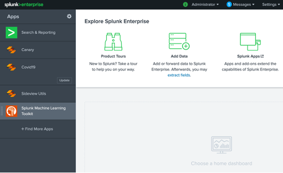
From the Apps interface, select Splunk Machine Learning (Figure 1).
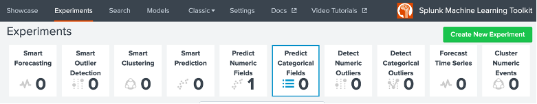
Figure 1: Splunk Apps We will now analyse a firewall log for malware. For this select “Predict Numeric Fields”, and then “Create New Experiment”:
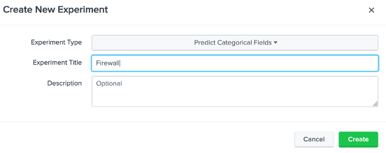
Figure 2: Selecting a Predict Categorical Fields experiment Provide the name of “Firewall” to the experiment title (Figure 3).
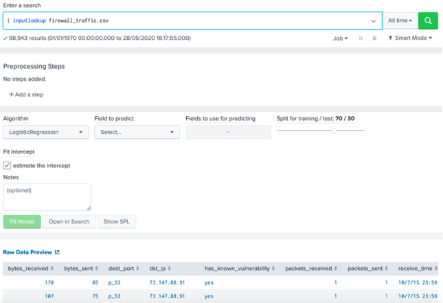
Figure 3: Defining a new experiment Next (Figure 4) entered the search of “| inputlookup firewall_traffic.csv” and select the green search button. It will then populate the data set in the page. Scroll down to the populated dataset and define the following: Number of results in the dataset: Parameters used in the dataset: Which field do you think we are likely to train on: Outline four IP addresses for source addresses: Outline four IP addresses for destination addresses:
Figure 4: Defining the dataset There are 98,943 results, which is rather large for processing so reduce it to 50,000 (Figure 5).
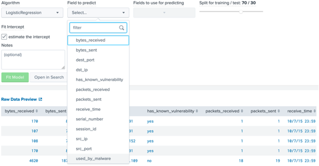
Figure 5: Filtering to 50,000 records Next we will use Logistic Regression to predict a value for “used_by_malware” (Figure 6). Which values are possible for the “used_by_malware” parameter?
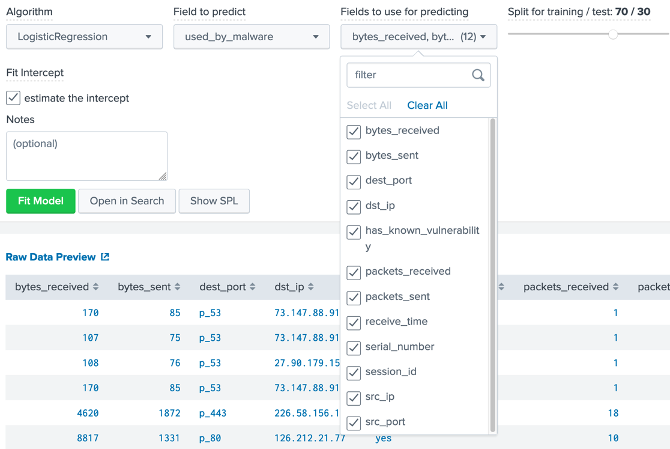
Figure 6: Predicting for “used_by_malware” Next we shall train against all the other parameters (Figure 7). Finally we are using a 70/30 split, and 70% of training and 30% for testing the model created.
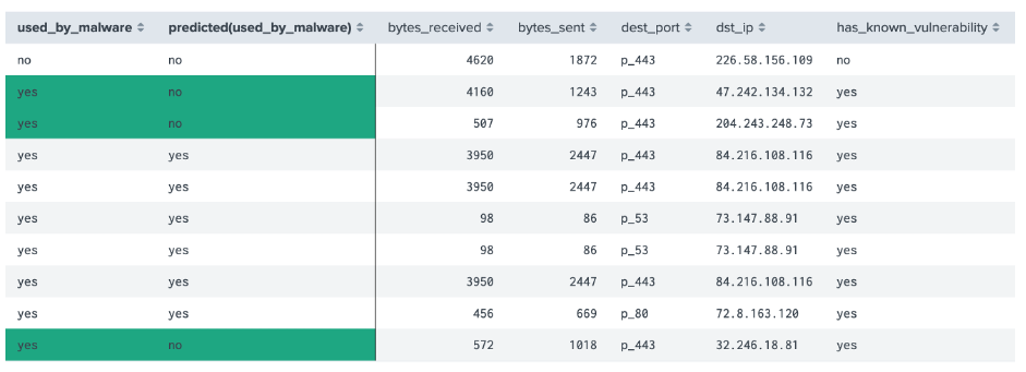
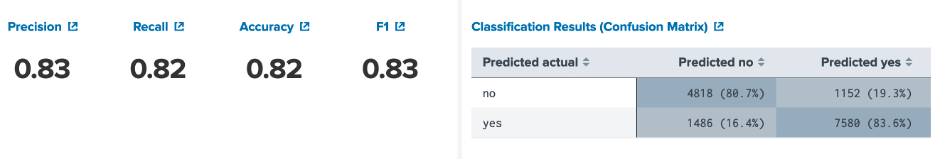
Figure 7: Fields used to predict Finally, we select the “Fitting Model..” button, and waiting until the model is built. When complete we should see prediction data (Figure 8). Outline the destination IP addresses for two false positives: Outline the destination IP addresses for two true positives: Now outline the following: Precision: Recall: Accuracy: F1: Outline the confusion matrix:
Figure 8: Predictions
Figure 9: Confusion Matric
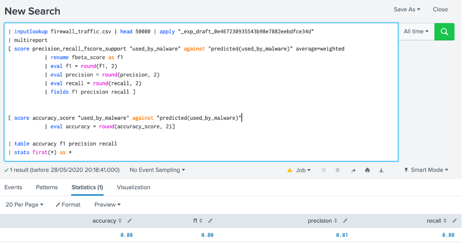
Figure 10: Confusion Matric Now click on “Open Search” in the button beside “Fit Model”, and enter the text in italic: Next press SHIFT-ENTER, and force the “| fit …” to move to the next line:
| multireport
[ score precision_recall_fscore_support "used_by_malware" against "predicted(used_by_malware)" average=weighted
| rename fbeta_score as f1
| eval f1 = round(f1, 2)
| eval precision = round(precision, 2)
| eval recall = round(recall, 2)
| fields f1 precision recall ]


[ score accuracy_score "used_by_malware" against "predicted(used_by_malware)"
| eval accuracy = round(accuracy_score, 2)]

| table accuracy f1 precision recall
| stats first(*) as *
This should give the output in Figure 11. Run the result and check the output. What are the results:
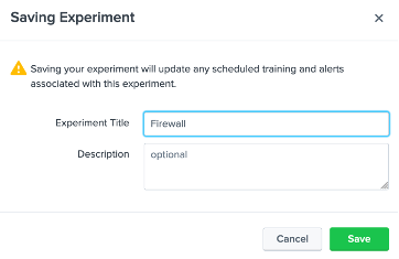
Figure 11: Update Finally save the experiment (Figure 12).
Figure 12: Saving experiment SVMWe will now use an SVM (Support Vector Machine) model and which is a supervised learning technique. Overall, it is used to create two categories, and will try to allocate each of the training values into one category or the other. Basically, we have points in a multidimensional space, and try to create a clear gap between the categories. New values are then placed within one of the two categories. In this case we will train with SVM, and rerun the model. Now determine the following: Precision: Recall: Accuracy: F1: Additional code| inputlookup firewall_traffic.csv | head 50000 | apply "_exp_draft_0e467230935543b98e7882eebdfce34d" | table "used_by_malware", "predicted(used_by_malware)", "bytes_received" "bytes_sent" "dest_port" "dst_ip" "has_known_vulnerability" "packets_received" "packets_sent" "receive_time" "serial_number" "session_id" "src_ip" "src_port" | inputlookup firewall_traffic.csv | head 50000 | fit SVM "used_by_malware" from "bytes_received" "bytes_sent" "dest_port" "dst_ip" "has_known_vulnerability" "packets_received" "packets_sent" "receive_time" "serial_number" "session_id" "src_ip" "src_port" into "_exp_draft_0e467230935543b98e7882eebdfce34d" | inputlookup firewall_traffic.csv | head 50000 | fit RandomForestClassifier "used_by_malware" from "bytes_received" "bytes_sent" "dest_port" "dst_ip" "has_known_vulnerability" "packets_received" "packets_sent" "receive_time" "serial_number" "session_id" "src_ip" "src_port" into "_exp_draft_0e467230935543b98e7882eebdfce34d" | inputlookup firewall_traffic.csv | head 50000 | fit GaussianNB "used_by_malware" from "bytes_received" "bytes_sent" "dest_port" "dst_ip" "has_known_vulnerability" "packets_received" "packets_sent" "receive_time" "serial_number" "session_id" "src_ip" "src_port" into "_exp_draft_0e467230935543b98e7882eebdfce34d" Tutorial 1The figure below outlines the access to Splunk for machline learning. For this select the link below and enter your username and password: http://asecuritysite.com:8443
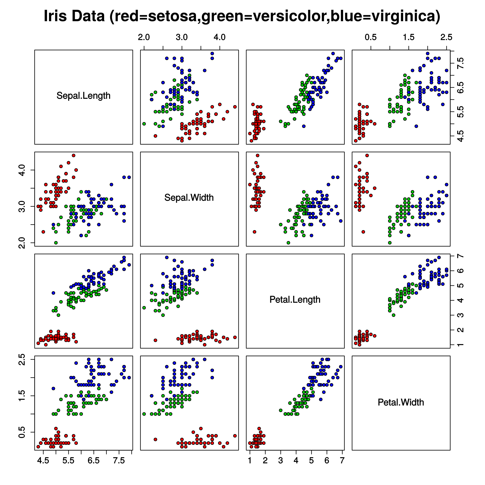
Anomaly DetectionIn this section we will analyse some of the models used to detect anomalies. The figure below outlines the mapping of the Iris dataset. The dataset contains four types of flower, and which have different dimensions for the petal length, petal width, septal length and septal width.
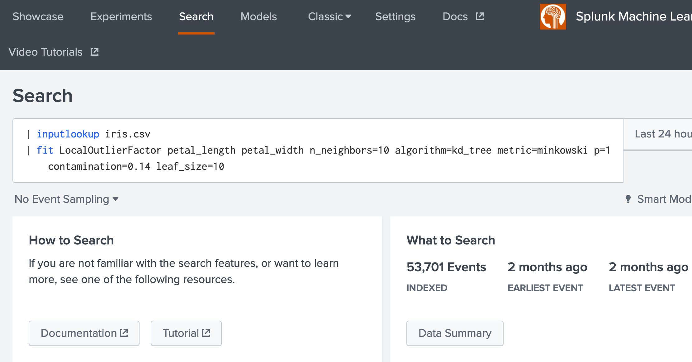
1. Select the Search tab, and in the search facility, enter the following [here]: | inputlookup iris.csv | fit LocalOutlierFactor petal_length petal_width n_neighbors=10 algorithm=kd_tree metric=minkowski p=1 contamination=0.14 leaf_size=10
How many records are there?
2. Next we will run a One Class SVM model for anomaly detection [here: | inputlookup iris.csv | fit OneClassSVM * kernel="poly" nu=0.5 coef0=0.5 gamma=0.5 tol=1 degree=3 shrinking=f into TESTMODEL_OneClassSVM
How many records are there?
3. We now will use a new data setup (call_center.csv) and run the Density Function method [here]: | inputlookup call_center.csv | fit DensityFunction count by "source" into mymodel
How many records are there?
Prediction (Categories)4. We will go back to our Iris dataset, and run AutoPrediction [here]: | inputlookup iris.csv | fit AutoPrediction random_state=42 petal_length from * max_features=0.1 into auto_classify_model test_split_ratio=0.3 random_state=42
Can you now train for sepal_length using sepal_width and petal_length. Outline one prediction for sepal_length (and the error from the actual value):
5. Now apply the BernoulliNB prediction model [here]: | inputlookup iris.csv | fit BernoulliNB petal_length from * into TESTMODEL_BernoulliNB alpha=0.5 binarize=0 fit_prior=f
Can you now train for petal_length using sepal_width and species. Outline one prediction for petal_length (and the error from the actual value):
6. Now apply the DecisionTreeClassifier prediction model [here]: | inputlookup iris.csv | fit DecisionTreeClassifier petal_length from * into sla_ MOD
Can you now train for petal_length using petal_width and species. Outline one prediction for petal_length (and the error from the actual value):
7. Now apply the GaussianNB [here]: | inputlookup iris.csv | fit GaussianNB petal_length from * into MOD
Can you now train for petal_length using petal_width and species. Outline one prediction for petal_length (and the error from the actual value):
8. Now apply the GradientBoostingClassifier [here]: | inputlookup iris.csv | fit GradientBoostingClassifier petal_length from * into MOD
Can you now train for petal_length using petal_width and species. Outline one prediction for petal_length (and the error from the actual value):
Prediction (Numeric)9. In the following we will use the track_day.csv data source. Perform an AutoPrediction model on batteryVoltage using longitudeGForce, speed and verticalGForce [here]: | inputlookup track_day.csv | fit AutoPrediction batteryVoltage target_type=numeric test_split_ratio=0.7 from * into PM
Outline some of the features within the track_day data set:
10. Perform an DecisionTreeRegressor model on batteryVoltage using longitudeGForce, speed and verticalGForce [here]: | inputlookup track_day.csv | fit DecisionTreeRegressor batteryVoltage from * into PM
Outline one prediction for batteryVoltage (and the error from the actual value):
11. Perform an ElasticNet model on batteryVoltage using longitudeGForce, speed and verticalGForce [here]: | inputlookup track_day_missing.csv | fit ElasticNet batteryVoltage from * into EN
Outline one prediction for batteryVoltage (and the error from the actual value):
12. Perform an GradientBoostingRegressor model on batteryVoltage using longitudeGForce, speed and verticalGForce [here]: | inputlookup track_day_missing.csv | fit GradientBoostingRegressor batteryVoltage from * into GB
Outline one prediction for batteryVoltage (and the error from the actual value):
Clustering13. In the following we will use the iris.csv data source. Perform Birch clustering model on petal_length for three clusters [here]: | inputlookup iris.csv | fit Birch petal_length k=3 partial_fit=true into MOD2
Outline one value from each cluster:
14. In the following we will use the iris.csv data source. Perform DBSCAN clustering model on petal_length for three clusters [here]: | inputlookup iris.csv | fit DBSCAN petal_length min_samples=4
How many clusters have been created:
15. In the following we will use the iris.csv data source. Perform GMeans clustering model on petal_length for three clusters [here]: | inputlookup iris.csv | fit GMeans petal_length random_state=42 into MOD3
How many clusters have been created:
16. In the following we will use the iris.csv data source. Perform GMeans clustering model on petal_length for three clusters [here]: | inputlookup iris.csv | fit KMeans petal_length k=3 into MOD4
How many clusters have been created:
Feature Extraction17. In the following we will use the FieldSelector method to determine the best feature selector for batteryVoltage given engineCoolantTemperature, engineSpeed, lateralGForce,longitudeGForce, speed [here]: | inputlookup track_day.csv | fit FieldSelector batteryVoltage from engineCoolantTemperature, engineSpeed, lateralGForce,longitudeGForce, speed type=numeric
Best feature:
18. Now we find the best feature for batteryVoltage for engineSpeed, lateralGForce and longitudeGForce [here]: | inputlookup track_day.csv | fit FieldSelector batteryVoltage from engineSpeed, lateralGForce,longitudeGForce, speed type=numeric
Best feature:
19. Now for vechicleType (and which is a category), determine its best match for engineCoolantTemperature, engineSpeed, lateralGForce,longitudeGForce, and speed [here]: | inputlookup track_day.csv | fit FieldSelector vehicleType from engineCoolantTemperature, engineSpeed, lateralGForce,longitudeGForce, speed type=categorical
Best feature:
20. Within the best feature, we can use the HashingVectorization to analyse the difference between strings (using N-grams). Run the following search [here]: | inputlookup passwords.csv | fit HashingVectorizer Passwords ngram_range=1-2 k=10
What is the data used in the dataset
21. The ICA (Independent component analysis) method is used to reduce the number of dimensions in the data. Run the following search [here]: | inputlookup track_day.csv | fit ICA batteryVoltage, engineSpeed, engineCoolantTemperature n_components=2 as IC
What do you observe from the output:
22. We can do the same reduction with PCA. Run the following search [here]: | inputlookup track_day.csv | fit KernelPCA batteryVoltage, engineSpeed, engineCoolantTemperature k=2 gamma=0.001 as PCA
What do you observe from the output:
23. NPR (Normalized Perlich Ratio) is useful in converting categorical fields into numeric values [here]: | inputlookup track_day.csv | fit NPR vehicleType from engineSpeed as npr01
What do you observe from the output:
24. Principal Component Analysis (PCA) reduce the number of fields in the data. Run the following search [here]: | inputlookup track_day.csv | fit PCA engineCoolantTemperature, engineSpeed, lateralGForce,speed k=2 as pca01
What do you observe from the output:
25. TF-IDF (Term Frequency-Inverse Document Frequency) converts raw text data into a matrix, and can be used to find words within documents. Run the following search [here]: | inputlookup track_day.csv | fit TFIDF vehicleType ngram_range=1-2 max_df=0.6 min_df=0.2 stop_words=english as tf01
What do you observe from the output:
Feature Extraction25. We can Imputer to replace data that is missing. Enter the following search [here]: | inputlookup track_day_missing.csv | fit Imputer batteryVoltage
What data has been replaced:
26. RobustScaler scales to median and interquartile range to 0 and 1. It thus reduces the bias caused by large data ranges swamping smaller values. | inputlookup track_day_missing.csv | fit RobustScaler *
Outline the result:
27. Now try the ScandardScalar [here]: | inputlookup track_day_missing.csv | fit StandardScaler * Forecasting28. A common method we have is to forecast over time. The StateSpaceForecast method is based on Kalman filters. Run the following query [here]: | inputlookup app_usage.csv | fit StateSpaceForecast CRM ERP Expenses holdback=12 into SF
Outline the result:
29. Finally, we can use the ARIMA model for forecasting. Perform the following search [here]: | inputlookup logins.csv | fit ARIMA _time logins holdback=0 conf_interval=95 order=0-0-0 forecast_k=5 as AR
Outline the result:
References[1] https://en.wikipedia.org/wiki/Iris_flower_data_set |